In order to calibrate the wetland, a gauge must be assigned to the RouteWetland Command. This can be done by right clicking the RouteWetland and selecting Has Gauge Here.

Then click the Plot Calibration button in the Simulation ribbon.

This will open the calibration window. Here you must add your monitored wetland surface water level.

Monitoring data should be saved as a CSV file with the file format show below. For this exercise, you can find the observation data files for each year in the folder “…\data” and the CSV file names are “SW40-1 Water Level – 2013.csv”, “SW40-1 Water Level – 2014.csv” and “SW40-1 Water Level – 2015.csv”.

To add calibration data to the Compared to Observed Data window, click Add… button. In the pop-up window, navigate to and double-click the observation data CSV file. The observation data will be added to Observed Data panel.

Then, drag and drop the added observation data from Observed Data panel to the right side of the window.

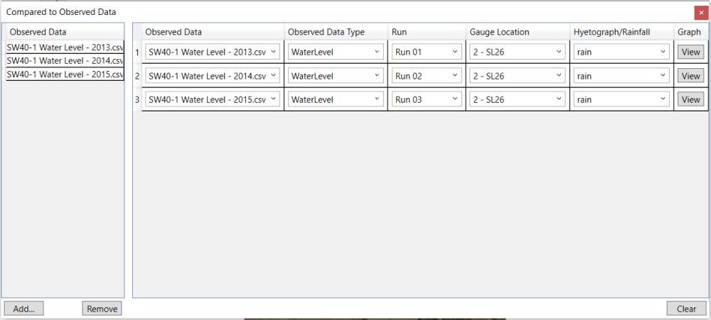
Select from the drop-down lists for each column in the window. Select “WaterLevel” as the Observed Data Type, “Run 01” as the Run to compare with Observed Data “SW40-1 Water Level – 2013.csv”, and “rain” as Hyetograph/Rainfall.

Follow the same way to setup the calibration comparison for each run as the figure below.

Click View after each comparison row to see the simulation vs observation comparison. This will display the monitored surface water level (green), the groundwater level (blue) and the modelled output surface water level (red). Below the graph, there is a Time Series Summary table and a Statics table. Click on the tab name to see each table.

You can now adjust your parameters to calibrate the model. It is suggested to keep values within +/- 20% of anticipated values. Check with your local approval agency to determine what they require as acceptable calibration values. It is suggested to match volumes to within +20% and -10%, match peaks to within +25% and -15%, visually match peak timing, and have an R2>0.70 and a Nash-Sutcliffe Efficiency >0.65.


