
In Canada, the Atmospheric Environment Service (AES) of Environment Canada does the collection of rainfall records. The rainfall amounts are collected using a tipping bucket rain gauge. The rain gauge typically records every 0.01 inches of rainfall. The AES standard procedure locates a Type B Standard Rain Gauge (AES standard) together with the tipping bucket and adjusts the tip-ping bucket data so that the daily totals of both gauges agree. In the United States the U.S. Weather Service collects data which is then stored and analyzed at the National Climate Centre (NOAA, Environmental Data Service Ashville N.C.). Worldwide meteorological information may be obtained from the World Meteorological Organization.
The AES analyzes the daily records obtained from the tipping bucket rain gauge. In the case of strip charts, these are analyzed to determine the maximum rainfall volume occurring in 5, 10, 15, 30, 60, 120, 360, 720, and 1440-minute intervals during each day of a year. The daily record of maximum volumes is scanned at the end of each year to determine the annual maximum volumes for each of the time periods. This analysis is conducted for every year of the rainfall record to form an annual maximum series. Each set of volumes is divided by the appropriate fixed duration to obtain the annual maximum series for intensities.
The return period of extreme intensities is of special interest to engineers who want to calculate the return period of the rainfall-induced peak flows. The return period can be determined using a plotting position formula or by using an extreme-value distribution. For example, the Atmospheric Environment Service uses the extreme value type 1 distribution. The statistical parameters of mean, standard deviation and skew are computed for each set of annual maximum intensities. The intensity of a particular frequency is computed using the statistical parameters and the frequency factor form of the probability distribution (Chow,1954). For each duration, the intensities for the desired return periods are computed. The points of intensity and duration for known return periods are plotted. Lines joining all the points having the same return period are drawn to form an IDF curve. An example of the intensity-duration-frequency (IDF) curves developed by the AES for the Bloor Street station in Toronto are shown in the figure below.
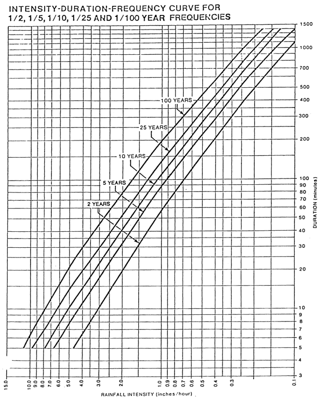
BLOOR ST. STATION
Engineers have also found advantageous to fit empirical equations to the statistically developed IDF curves. Equations 35 and 36 are the general forms of the empirical equations used most frequently.
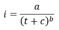 (35)
(35)
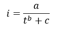 (36)
(36)
To describe the variation in average intensity with duration for a given frequency, the parameters a, b and c must be determined. This is done by fitting the either of the two equations to the statistically determined values for i and t. The value of b is estimated, then the following equation can be solved for the constants c and ln(a).
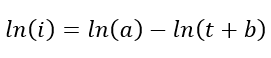 (37)
(37)
The values of a, b and c are unique for each IDF curve. They cannot be used to develop IDF curves of different frequencies or IDF curves at different locations.