
Click on the Existing scenario tab to show the Schematic view of the existing scenario, because we will use the Existing scenario for model calibration.
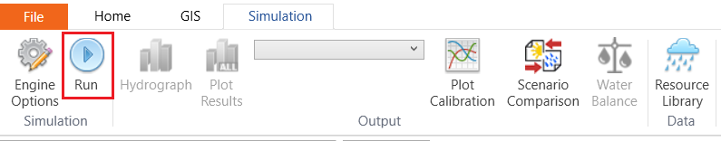
Click the Run button located at the Simulation tab.
In the opened Batch Run window, make sure your setting is as below. You can use Add button  or Remove button
  to add or remove runs. Click on the cell of name under the Name column to change the run name to “Calibration”.

Click on the Simulation Engine button  on the toolbar of the Batch Run window to open the Simulation Engine window.

On the Simulation Engine window, click on the Time Step tab and set the Simulation Time Step (min) as 5 min. Click OK to save and close the Simulation Engine window.

Click the Run button on the Batch Run window to run the model. Notice that a progress bar is given to show the progress and a message window is given upon the successful completion of the run.

Select the RouteChannel on Schematic view. Right-click to open context menu and then select Has Gauge Here.

Click Plot Calibration button in the Simulation toolbar.

In the pop-up window, click the Add… button to add the calibration data “…/data/calibration/calibration_flow.csv” to Observed Data panel.

Then, drag and drop the added observed data from the Observed Data panel to the right-side window. Set up the comparison as below.

Click the View button to see the comparison. On the Observed/Simulation Plot window, click the tabs “Time Series Summary* and Statistics below the graph to see summary and statistic tables.

You can also zoom into a timeslot by scrolling your mouse wheel or drawing a rectangular on the observation/simulation comparison graph to see more details at that timeslot.

You can now adjust your parameters to calibrate the model. It is suggested to keep values within +/- 20% of anticipated values. Check with your local approval agency to determine what they require as acceptable calibration values. It is suggested to match volumes to within +20% and -10%, match peaks to within +25% and -15%, visually match peak timing, and have an R2>0.70 and a Nash-Sutcliffe Efficiency >0.65.