Filter Strips
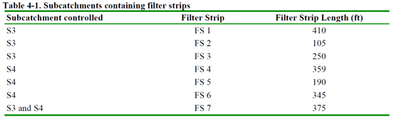
Figure 4-1 presentes the locations of the filter strips (FS) for this example. We’ll add these Low Impact Developments (LIDs) to the initial VOSWMM model, Example2-Post.inp, which already contains subcatchments and a runoff system. To assist in placement, we’ll use Figure 4-1 as a background image named Site-Post-LID.jpg. Table 4-1 specifies the subcatchment for each filter strip and its length.
Note:
An alternative to modeling Low Impact Developments (LIDs) without creating additional subcatchments is to use Sub-Area Routing in VOSWMM. In VOSWMM, each subcatchment consists of two sub-areas: impervious and pervious. You can choose from three Sub-Area Routing options: Outlet, Pervious, and Impervious.
- Outlet (a) routes runoff from both sub-areas directly to the subcatchment’s outlet.
- Pervious (b) routes impervious runoff across the pervious sub-area before reaching the outlet.
- Impervious (c ) routes pervious runoff across the impervious sub-area before reaching the outlet.
When impervious runoff is routed through the pervious area (b), some infiltrates and is stored in the pervious sub-area. The graph demonstrates how these methods affect runoff in a single subcatchment. Note that when pervious area runoff is negligible, the “100% routed to Outlet” and “100% routed to Impervious” cases yield similar results.

The Sub-Area Routing – Pervious option can model LIDs by representing the LID as the pervious sub-area, matching subcatchment pervious parameters with LID characteristics, routing impervious runoff to the pervious sub-area, and defining Percent Routed to show the percentage of impervious area connected to the LID. This method assumes the entire subcatchment’s pervious area represents the LID but lacks flexibility since it requires the LID to conform to the subcatchment’s slope and width, which may not always align with LID design needs.
We’re creating filter strips labeled as FS with numbers, and some will be grouped together as new subcatchments named “S_FS_number.” (Table 4-1).
To improve our runoff estimates for the filter strips, we’re further dividing subcatchments S3 and S4 into smaller parts, such as S3.1, S3.2, and S4.1, as shown in Figure 4-4. This means re-evaluating runoff lengths, subcatchment widths, slopes, and impervious percentages. For guidance on determining these properties, refer to Example 1.
The new subcatchments representing lots will have a 2% slope. We’ll continue using the same Horton infiltration rates as in previous examples: 4.5 in/hr for the maximum, 0.2 in/hr for the minimum, and 6.5 hr-1 for the decay constant.
To accommodate these new subcatchments and improvements, we’re introducing new channels and junctions connecting them to the drainage system, depicted in Figure 4-4 (pipes in red, junctions in blue). See Table 4-2 for the properties of the new junctions and Table 4-3 for the new conduits.
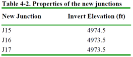
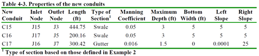

Figure 4-4
Table 4-4 summarizes the properties of the new subcatchments. It’s worth noting that the outlets of some new subcatchments (S3.2, S3.3, S4.2, and S4.3) are not junctions but filter strips represented as subcatchments. Figures 4-5 and 4-6 illustrate this layout within the SWMM model.
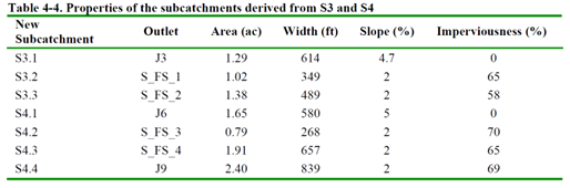
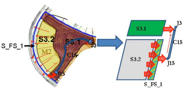
Figure 4-5
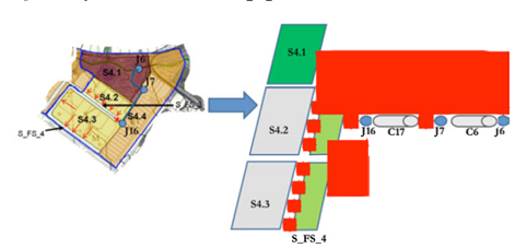
Figure 4-6
For the filter strips, the overland flow length will be 4 feet, with a slope matching the typical lot slope of 2%. The strip widths, perpendicular to the flow direction, have been directly measured from the map using the Ruler tool, as explained in Example 1, and are detailed in Table 4-5.
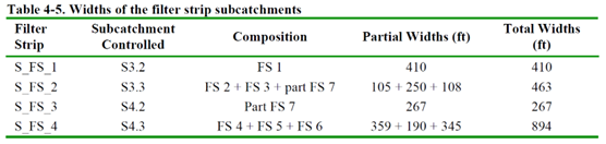
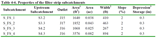
Table 4-6 summarizes the characteristics of the subcatchments used for modeling the filter strips in this example. The filter strip areas are calculated based on their measured lengths and a fixed flow path length of 4 feet.
Once we’ve added the filter strip properties from Tables 4-5 and 4-6 to the model, all filter strips are given the following attributes:
- Zero percent imperviousness
- Impervious roughness of 0.015 (although not used due to 0% imperviousness)
- Impervious depression storage of 0.06 in (not used due to 0% imperviousness)
- Pervious roughness of 0.24
- Pervious depression storage of 0.3 in
Both maximum and minimum infiltration rates for Horton infiltration are set to 0.2 in/hr, representing the minimum soil infiltration rate in the area. This conservative approach accounts for potential infiltration capacity losses and possible soil saturation at the start of a new storm.
Every subcatchment in the SWMM model requires a rain gauge assignment. However, since no rain should fall on the filter strip subcatchments (as they are part of other subcatchments), we create a “Null” Time Series with a single time and zero rain value. A new rain gauge named “Null” is linked to this “Null” time series and serves as the rain gauge for all filter strip subcatchments. Subcatchments generating runoff are connected to the original “RainGage,” as in previous examples.
Infiltration Trenches
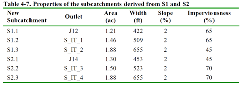
In this example, we have infiltration trenches (IT) located in the northern part of the study area, as shown in Figure 4-1. To model these, we first divide subcatchments S1 and S2 into six smaller subcatchments, as seen in Figure 4-7. Imperviousness for each subcatchment is determined by the land use type (M, L, or DL) from Table 1-6 in Example 1. Table 4-7 summarizes the properties of these subdivided subcatchments. Other properties, such as Horton infiltration and pervious depression storage, remain the same as the original subcatchments.

Figure 4-7
The infiltration trenches are listed in Table 4-8, labeled IT with numbers, and their locations are shown in Figure 4-7. These trenches are incorporated as subcatchments with names prefixed by S_. They serve as outlets for subcatchments S1.2, S1.3, S2.2, and S2.3, as indicated in Table 4-9. Subcatchments S1.1 and S2.1 use junctions J12 and J14 as outlets.
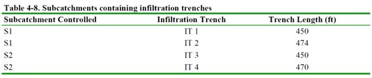
For sizing the infiltration trenches, note that the definitions of length and width are opposite to those for filter strips. Table 4-8 provides trench lengths, and their areas can be calculated with an assumed width of 3 ft. Widths and areas for each trench are detailed in Table 4-9. Each trench is modeled with a depression storage depth of 1.2 ft, with infiltration below this depth and flow along the trench above it. While the actual storage depth of the trenches is 3 ft, the effective storage depth for infiltrating water is reduced to 40% of the actual depth due to the 40% porosity of the 1-1/2 in. diameter gravel in the trenches. Table 4-9 summarizes properties assigned to the trench subcatchments.
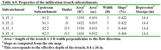
Trench slopes are directly derived from the site map, and imperviousness is set at 0%. Manning’s roughness coefficient is 0.24, and depression storage is configured as an effective storage depth of 14.4 in (1.2 ft). Similar to the filter strips, a constant (minimum) soil infiltration capacity of 0.2 in/hr is used for the trenches, without considering horizontal infiltration through trench sides. Each trench subcatchment uses the “Null” rain gauge to prevent direct rainfall over the trench area.
This design assumes no barriers affect water flow into the trench. For instance, a layer of grass and soil above the 1-1/2 in. diameter gravel might slow flow into the trench, resulting in less treated flow. This aspect will be explored further in the results section.
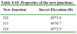
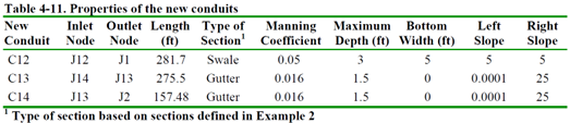
To complete the model, additional channels and junctions connecting the new subcatchments to the drainage system are defined, as illustrated in Figure 4-7 (red conduits and blue junctions). Table 4-10 provides properties for the new junctions, and Table 4-11 details the new conduits.