We ran both the EMC washoff model (Example5-EMC.inp) and the exponential washoff model (Example5-EXP.inp) for 0.1 in., 0.23 in., and 2-year rainfall events, with the following analysis options:
| Simulation Period: | 12 hours |
| Antecedent Dry Days: | 5 |
| Routing Method: | Dynamic Wave |
| Routing Time Step: | 15 seconds |
| Wet-weather Time Step: | 1 minute |
| Dry-weather Time Step: | 1 hour |
| Reporting Time Step: | 1 minute |
EMC Washoff Results
These concentrations are constant, comprising the rain’s consistent concentration (10 mg/L) and the EMCs assigned to each subcatchment’s land uses. When surface runoff ends, TSS concentration drops to zero. Subcatchment S7, with no runoff (all rain infiltrated), has no displayed concentration. Notably, with EMC washoff, storm size doesn’t affect subcatchment runoff concentration.
The TSS concentration over time (pollutograph) at the study area outlet for the 0.1 Design Storm, 0.23 Design Storm, and 1.0 in. storms. It reflects the combined impact of TSS washoff from each subcatchment and conveyance network routing. While pollutograph peak concentrations and shapes are similar, outlet concentrations decrease over time. This is mainly due to the longer time for runoff from subcatchments with lower EMCs (e.g., S3 and S4) to reach the outlet. Some attenuation also arises from numerical dispersion, assuming complete mixing within conveyance conduits during pollutant routing.
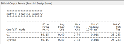
TSS concentrations continue to appear at the outlet even after the storm has ended. This is because conduits still carry a small volume of water with high EMC levels due to the flow routing process. However, it’s essential to note that these apparent high concentrations translate into negligible pollutant loads. This can be observed when comparing the outlet hydrograph and loadograph for a specific storm event, like the 0.1 inch event. The loadograph represents the product of concentration and flow rate over time. In this case, the loadograph was created by exporting relevant data into a spreadsheet, where flow and concentration were multiplied (converted to lbs/hr), and both flow and load were plotted against time. It’s evident that the TSS load discharged from the catchment decreases similarly to the total runoff discharge.
Understanding Water Quality Information in the VOSWMM Output Results
Water quality simulation in VOSWMM is available on the output results with four general sections (A, B, C, and D). We’ll explore these additions using Example5-EMC.inp and the 0.1 inch precipitation event as an example.
Part A in the report outlines the overall water quality balance in the study area. “Input” loads encompass Initial Buildup before the simulation, Surface Buildup during dry weather, and Wet Deposition from rainfall pollutants. “Output” loads include Sweeping Removal (not simulated), Infiltration Loss (simulated automatically), BMP Removal (not considered here), and the pollutant load in Surface Runoff (comprising washed-off buildup, direct deposition, and runon loads). The report also shows Remaining Buildup.

Part B displays the quality-routing balance. Here, only runoff loads move through the conveyance system. Dry weather, groundwater, RDII, external inflows, treatment, and decay are not considered in this example. So, the summary focuses on just three variables: Wet Weather Inflow, External Outflow, and Final Stored Mass. Notably, the Wet Weather Inflow in Part B matches the Surface Runoff in Part A.

Part C offers an overview of the pollutant load washed off from each subcatchment. Among them, subcatchments S7 and S3 yield the least TSS loads. Subcatchment S7, as it doesn’t produce any runoff, generates no load. Meanwhile, S3, with a substantial pervious surface area, contributes a smaller load.

Part D shows the cumulative loads exiting the system via its outfalls.
Exponential Washoff Results
In the simulation, TSS concentrations in runoff from various subcatchments differ during the 0.1 inch storm, using the Exponential washoff equation. Unlike EMC results, these concentrations vary throughout the runoff event and depend on both runoff rate and remaining pollutant mass on the subcatchment surface. For the 0.23 inch storm, there are notable differences: TSS concentrations are much higher (about 10 times) and TSS generation is faster, as seen in sharper pollutograph peaks. For the larger 1-inch, 2-year storm, TSS concentrations are slightly larger than the 0.23 Design Storm but not as significant as the shift from the 0.1 inch to 0.23 inch storms. Similar patterns apply to pollutographs at the watershed’s outlet.
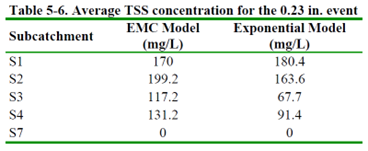
Although the EMC and Exponential washoff models use different coefficients that aren’t directly comparable, we calculated the average event concentrations for each subcatchment during the 0.23 design storm using both models (Table 5-6). The point is that, despite different-looking pollutographs, with suitable coefficient choices, you can achieve similar average event concentrations. While the Exponential model might seem more intuitive for pollutant washoff, without field measurements, it’s hard to claim it’s more accurate. Most SWMM modelers prefer the EMC method unless they have data to estimate and calibrate coefficients for a more advanced buildup and washoff model.