7.1 Examples of current methods

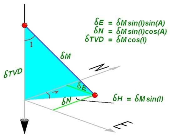
Over the years there have been several methods of calculating survey positions from the raw observations of measure depth, inclination and direction. At the simplest level if a straight line model is used over a length dM with inclination I and Azimuth A, we can derive a shift in coordinates as in below.

This simple technique is often referred to as the Tangential Method and is relatively easy to hand calculate. However, the assumption that the inclination and direction remain unchanged for the interval can cause significant errors to accumulate along the wellpath.

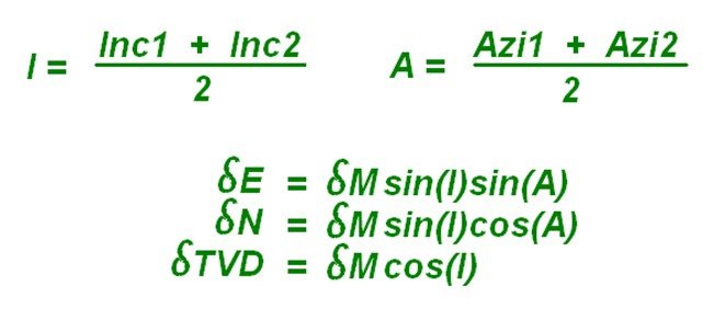
An improvement to this was the ‘Average Angle Method’ where the azimuth and inclination used in the above formulas was simply the average of the values at the start and end of the interval.

Average Angle Example

• Md1 = 1000 Inc1 = 28 Azi1 = 54
• Md2 = 1100 Inc2 = 32 Azi2 = 57
• Delta MD = 100
• Average Inc = 30
• Average Azi = 55.5
• Delta East = 100 sin(30) sin(55.5) = 41.2
• Delta North = 100 sin(30) cos(55.5) = 28.3
• Delta TVD = 100 cos(30) = 86.6

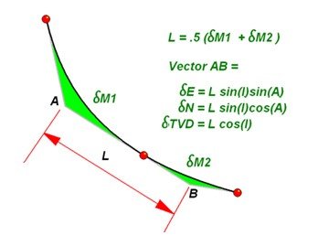
A further improvement was the Balanced Tangential Method whereby the angle observed at a survey station are applied half way back into the previous interval and half way forward into the next.

These techniques all suffer from the weakness that the wellpath is modelled as a straight line. More recently, the computational ability of computers has allowed a more sophisticated approach. In the summary below we see two curved models.

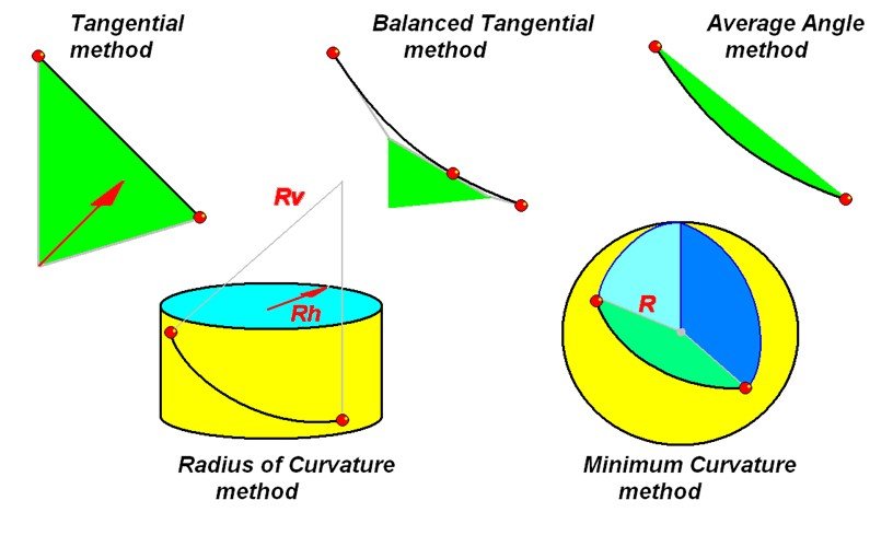
The one on the left assumes that the wellpath fits on the surface of a cylinder and therefore can have a horizontal and vertical radius. The one on the right assumes the wellpath fits on the surface of a sphere and simply has one radius in a 3D plane that minimizes the curvature required to fit the angular observations. This method, known as the ‘Minimum Curvature’ method, is now effectively the industry standard.

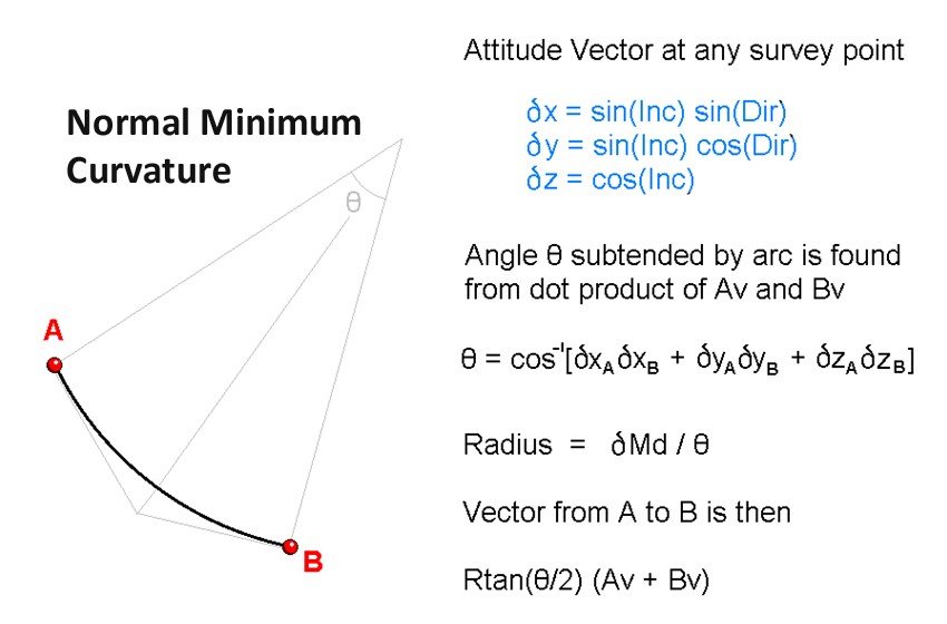
Imagine a unit vector tangential to a survey point. Its shift in x, y and z would be as shown above. The angle between any two unit vectors can be derived from inverse cosine of the vector dot product of the two vectors. This angle is the angle subtended at the centre of the arc and is assumed to have occurred over the observed change in measured depth. From this the radius can be derived and a simple kite formed in 3D space whose smaller arm length follows vector A then vector B to arrive at position B.

Notice however that the method assumes a constant arc from one station to the next and particularly when using mud motors, this is unlikely to be the case