14.1 Calculation and background

A more recent development on the principle of magnetic interference correction is the use of Multi Station Analysis.

This technique is similar to the rotational shot technique described above but makes use of all available MWD data so far collected to ‘best estimate’ corrections to apply retrospectively. This is heavy on computing time but with modern computers allows a great deal more flexibility in what we analyse for. In the section following the mathematics will be set out but for now, the principles and process steps are as follows.

Earlier we discovered that a magnetometer will read a magnetic field value along its own axis. It is therefore possible to calculate a theoretical value if we know the background field vector and the ‘attitude’ (Inclination and Direction) of the sensor axis. If we gather a lot of raw data from multiple survey stations (with the same BHA), we can examine the consistency of the data versus the theoretical values and try to find corrections on each sensor that make for the least error.

This is known as Multi Station Analysis and since it is using all the raw data over several stations, in theory, there is no need to carry out a cluster shot since there will be variations in attitude anyway between each survey station. It should be said however, that cluster shots are strongly recommended at the start of the BHA run to produce a strong estimate of corrections before drilling much further on what could be a wrong azimuth.

The steps are as follows:

1. Over several readings observe Bx, By, Bz, Gx, Gy and Gz
2. Calculate inclination, direction and toolface as normal
3. Calculate the unit vectors that describe the attitude of each magnetic sensor
4. Calculate the theoretical value that should have been read
5. Record the errors (residuals) on each sensor
6. Calculate the sum of the squares of these residuals
7. Try variations of scale and bias corrections on each sensor until the result of step 6 is minimised
8. Apply these best fit biases and scale factors over the whole survey

The next section may help the mathematicians amongst you understand the steps more clearly, and for the rest, may offer an alternative to counting sheep.

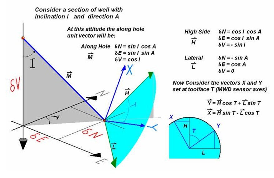
These formulae describe the high side unit vector and the lateral unit vector from which we can derive the axes vectors when sitting at any given toolface from high side;

If we describe the Earth vector in terms of a north, east and vertical component we can calculate theoretical readings for each axis using the vector dot product. If the Earth’s magnetic Field Vector os Mag N, Mag E, Mag V and the Earth’s Gravity Field Vector is Gn, Ge an Gv we would expect each sensor to read the vector dot products as follows;

In practice we usually ignore any Gn and Ge components and assume that Gv is the Gravity Gt;

Returning to our magnetic equations, the red numbers are now known;

Each sensor observation provides one equation;

These equations can be used to solve for sin A and cos A and thus an unambiguous best fit azimuth can be derived from the observations. The unit vectors can be calculated and the theoretical readings subtracted from the observed readings to produce residuals for each observation and each axis.

A ‘Monte Carlo’ analysis is then run for variations in scale factor and bias for each sensor until the sum of the residuals squared is minimized. In the following graphs for all 6 corrections, a clear minimum sum squared occurs at the best value for each correction:

All previous raw surveys up to that point are then corrected with this latest estimate and the azimuths recalculated as if there was no magnetic interference present.

In practice the data will be noisy and often requires some filtering before it can be used. Any bad readings are either weighted low in the least squares calculation or they are removed altogether.