19.2.6 Summing Error Terms and Propagation Modes

Once we have calculated the contribution to the error ellipse from each error source, at each survey station in each leg of our well we have to sum up all the contributions.

There are two basic cases:
*1) The contributions are directly linked *(correlated in mathematical terminology).For example; the z-axis magnetometer bias error. If we are using the same tool and BHA, then we would expect
this error source to have the same value from survey station to survey station and the effects of the error will build all the way down the wellbore.

In this case the error contributions are added in the usual arithmetic way:

2) The contributions are not linked at all (statistically independent).
For example; if we have two independent error sources, then they could both cause a positive inclination error and add together but it is also possible that one might create a positive inclination error and the other a negative error.
In which case we are taking a random value from pot 1 and a random value from pot 2 and the error contributions must be root sum squared (RSS) together:

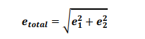
In fact, it is an assumption of the model that the statistics of the various different error sources are independent so they must be RSS’d together – for example, there is no reason why sag error would be connected to z-axis magnetometer bias or to declination error etc.

However, if we take the example from 1) above, although we can see that the z-axis magnetometer bias should remain the same throughout a survey leg, if we go to another leg, using a different tool or to another well then we would expect that error source to be independent over that range.

So far, the error sources are independent from each other, but a given error source might be independent at all times, or correlated from station to station within a survey leg or from survey leg to survey leg with a well or from well to well within a field.

Therefore, the model defines four *propagation modes *for the errors:

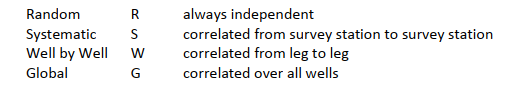
The propagation mode is a property of the error source and is defined in the tool model. In practice, most error sources are systematic or random and only a limited few well by well or global sources have been identified.

To combine all the error sources, we need to create a sum over all survey legs, survey stations and error sources which apply to a particular well. When doing this summation, the propagation mode is used to define at what step in the summation arithmetic addition is used and at what stage RSS addition is required.

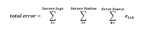
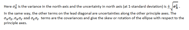
The mathematical details of this process can be found in Appendix A. The final output of the summation is a 3×3 covariance matrix, which describes the error ellipse at a particular station. In the nev-axes, the covariance matrix is: