
In reality this is a complex calculation best left to computer software but a very simple rule of thumb can estimate spatial error from an angular error as follows:
1 degree in angle creates about 2% in distance.
For example; if a line of 1000 m was measured on a bearing of 90 degrees plus or minus 1 degree, the final point would be in error by approximately +/- 2 0m.
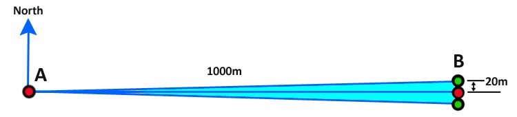
The correct answer would be closer to 1000 sin (1o) = 17.45m but as a conservative estimate the 2% per 1° rule is easy to calculate.
It is not true that errors are proportional to measured depth. In surveying, systematic (i.e. unchanging) errors propagate in proportion to how far you are from your origin. A compass reference error for example may pull you to the right as you walk away from the origin but will still pull you to the right as you return effectively cancelling out the positional error. A scaling error may underestimate your distance from the origin but equally it will be proportional to the distance and will cancel out on the return. When estimating the likely positional error, we can use this simple fact and the assumption that the dominant errors are systematic. Clearly though, not all errors are. Some errors like gyro drift are time dependent and therefore continue to get worse, the longer the route and others are random like the effects of inadequate survey intervals but we can still come up with a rough estimate that will allow us to assess the realism of any quoted error models and the likelihood of hitting a target.
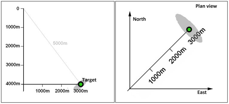
In this example a target is to be drilled with MWD with the following typical accuracies: measured depth is good to 2m/1000m, inclination to +/- 0.3° and azimuth to +/- 1°. Let’s try to work out the approximate ellipse of uncertainty by the time we reach the target.
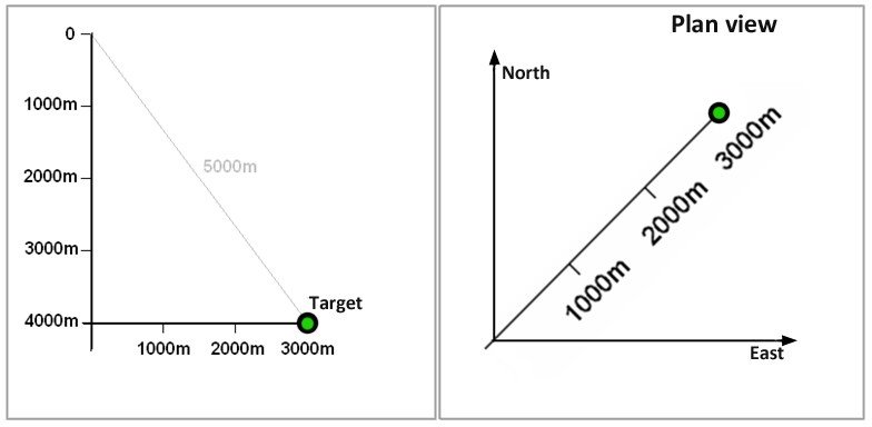
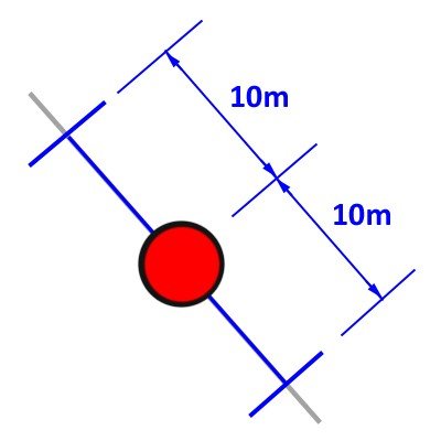
Firstly let’s determine the effect of the measured depth error of 2 m/1000. In this simple example, this can be determined without knowing the planned trajectory. The accumulated error at the target will be the same no matter what path we take to get there. This is not necessarily obvious. Using the fact that survey error propagates with distance from origin we can draw the uncertainty axis created by depth error as a line of 10 m (2m/1000m x 5000m distance) towards and away from the origin.
By way of example, if the well was drilled as a horizontal well with 4000 m vertical drilling and 3000 m horizontal drilling after a sharp build to horizontal, the total MD would be 7000 m. Let’s say that the depth was overshooting by 2 m/1000 m.
In this case, the depth error would be 2m/1000m x 7000m = +/-14m. If this had been a straight vertical well our depth could actually be anywhere between 6986 m and 7014 m.
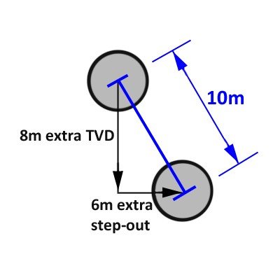
But in this case when we are only 5000 m from our origin our depth error at our presumed position is 2m/1000m x 5000m = +/-10m. Traveling to our target position would be to over/under shoot the vertical by 8 m and over/under shoot the horizontal by 6 m creating a positional error of 10 m on the axis shown above.
The effect of the inclination error can similarly be calculated using our simple rule. Inclination only affects the vertical plane and we are 5000 m from the origin in this plane so the positional error will be at right angles to our space vector and will have a magnitude of 0.6% of 5000 m or 30 m.
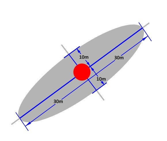
The third axis will be in the horizontal plane and is due to the azimuth error of 1°. This will produce an ellipse axis across the wellbore of approximately 2% of 3000 m which is 60 m. It is quite common for the azimuth error to be the dominant error in a 3D ellipse of uncertainty. These ellipses are not to scale but show the orientations and relative sizes.
Post your comment on this topic.