
The “Key Performance Indicator” (KPI) gives some statistics or key figures on the selected orders, projects or operations. It can be used to compare different planning scenarios in order to achieve the most optimal plan. Among others it shows the quantity of late and early orders and the average process- and lead time. The data in the two tables can be copied to a spread sheet by selecting the data with the mouse and doing a “ctrl+c and ctrl+v”.
The KPI dialog has three tabs, for showing statistics about Projects, Orders or Operations.
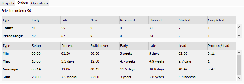
The KPI dialog
The KPI consists of two tables where the first one focuses on “count figures” and the last one focuses on “time figures”. The first one counts the quantity of early and late orders and it counts the quantity of the various states. The last table shows the min, max, average and sum values for the time figures.
Example of use
The various figures in the KPI can also be viewed in the “Order list” or “Project list”. In that way the details per order/project which consists of the basis for the statistics can also be viewed.
In the the example below the seven highlighted columns have been added to the “Order list” via the field chooser (right click on the table header to access the field chooser).
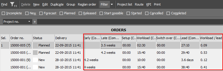
The list shows four orders where two are early and two are late.
In order to see the KPI for the orders select them all and click the highlighted “KPI” button.
KPI on the above four orders.
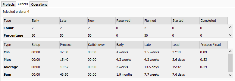
On the above example the min process time is 02:30. This can be identified in the “Order list” a little further up on order no. “15000-005 (7)” (workload = process). It is also illustrated that the max late time is 4.2 weeks. This can be identified in the “Order list” on order no. “15000-005 (15)”.
Operations tab
The operations tab shows pretty much the same indicators as the orders and projects tab. New indicators here are “Ahead” and “Behind”.
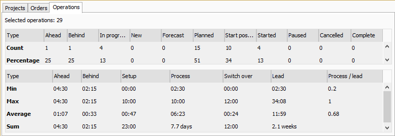
Notice that ahead and behind statistics is only based on operations in progress. On the above example there are selected 29 operations but there are only 4 operatons in progress (see “In progress” column). An operation is considered ahead schedule if it’s actual end calendar is before it’s planned end calendar.
The calculations
The calculations are performed by evaluating all the operations in the selected orders or projects. If the “Orders” tab is selected the statistics is performed per order – i.e. the average process time is calculated by summing the process time of all the operations and dividing by the number of selected orders. If the “Projects” tab is selected the calculations are performed per project – i.e. the average process time is calculated by summing the process time on all the operations and dividing by the number of selected projects. This will normally result in higher min, max and average figures on the “Projects” tab than on the “Orders” tab. However the “sum” figures will normally be the same on the two tabs – provided that the calculations are based on the same orders.
Setup, process and switch over
The approach for calculating the min, max, average and sum of setup, process and switch over is identical. In the following example the process time is calculated.
“Orders” tab:
First the process time per order is calculated by summing the operations in each order. Then the orders are evaluated where the min and max process time is identified. The average is found by dividing the sum of the process time by the number of orders.
Average process on orders = (Ʃ process) / “quantity of orders”.
“Projects” tab:
The process time per project is calculated. Then the projects are evaluated where the min and max process time is identified. The average is calculated by dividing the sum of process by the number of projects.
Average process on projects = (Ʃ process) / “quantity of projects”.
Early and late
The early and late time is found by subtracting the delivery time of the order/project by the latest operation’s end time. If the result is negative the order/project is late and vice versa.
Lead
The lead time is the duration of the order/project, i.e. the time from the first operation’s start time to the last operation’ end time in the order/project.
Process / lead
The “process / lead” can express the “efficiency” of the plan. It is calculated by dividing the process time of an order/project by the lead time. Thus the higher lead time the less “efficiency”. The higher process / lead time the better. If an order/project contains parallel operations the process / lead time can be greater than 1.
Consider the example below:
The order “15000-004” is illustrated below and contains two operations.
The first operation starts at Feb the 2nd at 10:00 and the last operation ends at Feb the 5th at 10:00, so the lead time is three days = 72 hours. The first operation has a process time on 5 hours and the last has 10 hours, thus the process time of the order is 15 hours.
Process / lead time = 15 hours / 72 hours = 0.2.
If the last operation was moved so it would begin just when the first operation ends, the process / lead time figure would be higher.
Post your comment on this topic.