Multiple Regression Analysis

For Video teaching on Market Models go here.

Definition: Multiple Regression Analysis (MRA) looks at the relationship between variables to PREDICT something.
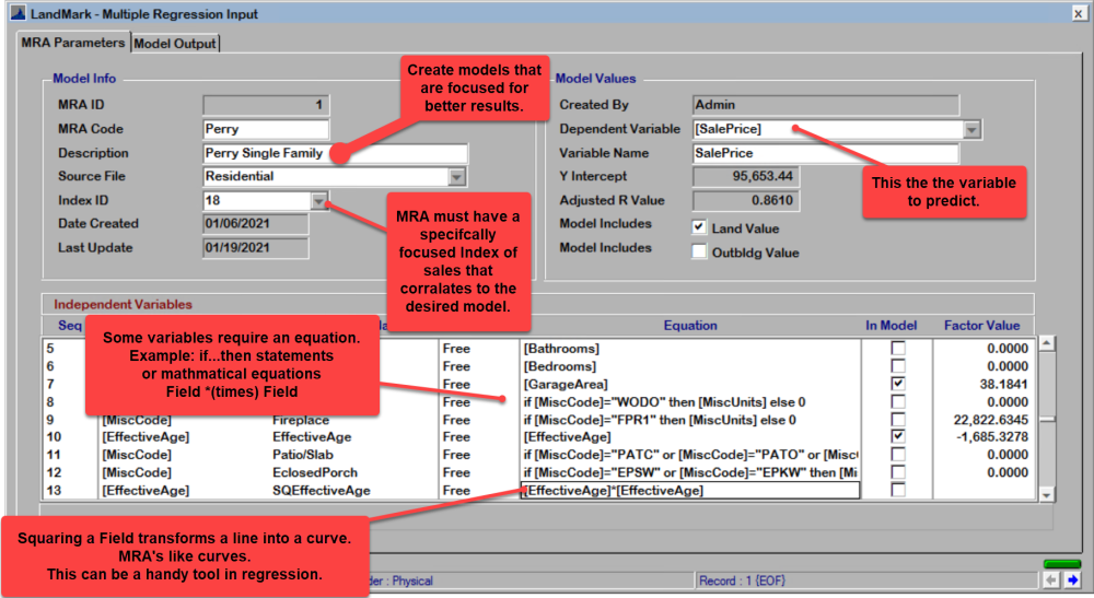
In appraisal it’s useful in predicting many things: property’s sales price, rent value, physical depreciation etc. A MRA can be focused or broad.

To View/Edit/Create New MRA Table from the Appraisal File go to:
Tables — Appraisal Tables — MRA Table
OR
From Main Menu — Appraisal — Appraisal Table — MRA Table

When building a Regression Model in LandMark user must do the following:

• Build an Index In the Appraisal Snapshot (to be assigned to MRA). Indexes can be as focused or diverse as you want the model to be.
  Example: If your MRA is built for the WHOLE county, be sure the Index draws parcel records from the whole county. If the MRA is built for single family properties in a particular small village, build an Index that pulls from that village (or neighborhood) only.
  Idea: Regression Analysis Models and Indexes may better if they are more focused.
  Example: Appraiser may want to build multiple, focused models to cover specific TYPES of properties or specific AREAS in the county.
• Build a Regression Model
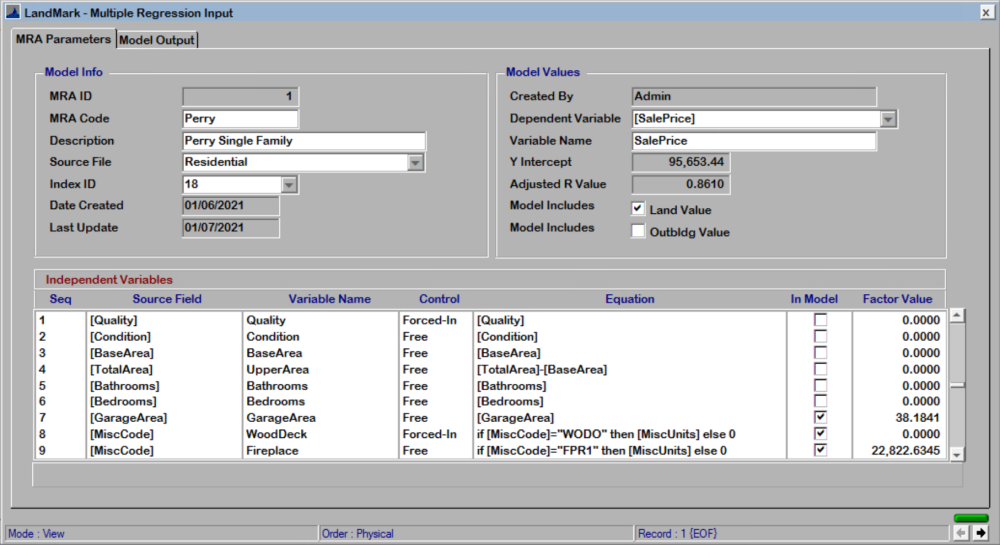
  (The example below shows a MRA for Single Family Residential properties in the town of Perry. There are no limits put on the house age or neighborhoods.)
  Helpful Hint: When building a MRA, use A LOT of variables. When many variables are used, the model itself will tell the user which variables have an impact on whatever user is looking for. (In this example, sales price.) In other words, the model will ask the system many questions. In return, the MR model will tell which variable(s) has an impact on value. TO INCLUDE SOMETHING AS A VARIABLE, USER SHOULD HAVE SEVEN TO EIGHT SALES THAT HAS THAT VARIABLE.
  

Independent Variables: aren’t correlated to each other, but they are correlated to the dependent variable

To run an MRA model that is built, go to:
Tools — Run Regression
This box will appear.

Output Types
None: no output
Spreadsheet: to view results in Excel
Text-File: shows the breakdown of the actual Regression Analysis

Regression Types
Best Fit: (linear) gives you one predicted model
Stepwise-Forward: (best to use) for every iteration (the repetition of a relationship of variables) it will find the variable with the MOST impact on value. The model will ADD that to the model and CHANGE the predicted values.

Maximum Probability to Enter: 0.05 (if the probability is higher than .05 it will enter the equation) .025
Minimum Probability to Retain: .10 (if the probability is lower than .10 it will leave the equation) .05
(If you make these smaller, you get more data.)

The check boxes will show the statistical breakdown in the text-file. CHECK the boxes important for data analysis.

CLICK RUN to run the analysis through the assigned Index.

The Text-File will appear.

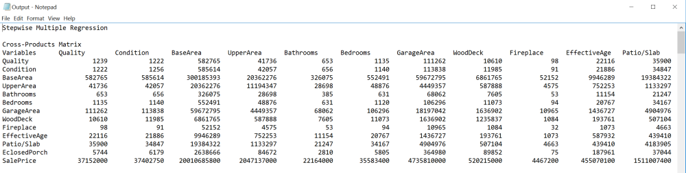
What the Text-File Data Means Overview

Correlations Matrix (Appraiser may want to look at this.) A good question to ask: Are properties correlated with the sales price (dependent variable) or something else?
Example: Bedroom count goes up as Base Area goes up. So if, BOTH areas come into the model.

Steps are the beginning of the Regression Analysis. They look for what has the most impact on sales price (dependent variable in this example).

Statistical Definitions As the model progresses goes through the steps, the numbers will change, hopefully becoming more ideal.

• The Adjusted R-Squared Value or Goodness of Fit In statistics, the adjusted R-squared shows whether adding additional predictors improve a regression model or not. It tells user if the variable is a good fit or how well it fits to a curve or a line. The higher the number gets, the more of the sale price our model explains. (Example: .6602 Isn’t good. Needs to be closer to 1.000—which is perfect.)

• Standard of Estimate of Error it is used to check the accuracy of predictions made with the regression line
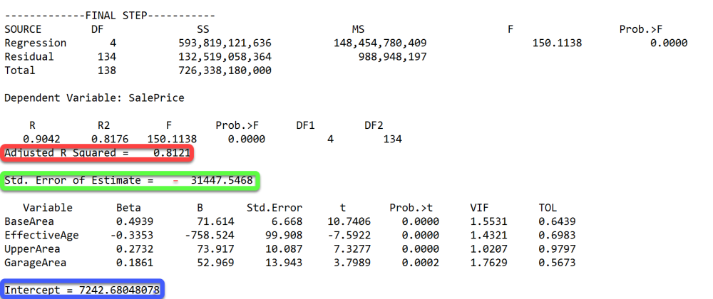
  In the example below: Starts at 46,238 and in the final step is at 31,447. (As an appraiser, in this example, you would want this number to be $20,000 or $15,000 would be even better.)

• Intercept or Constant (this is where adjustments start from)

• F-Stat or F To Enter the probability. This is the probability range limits the user set. It tells the next highest number candidate to come into the equation in next step. This will be the highest number in that column. The higher the number the more weight it is given compared to the dependent variable.

Transformation changing of a variable equation. Example: squaring the factor [EffectiveAge]*[EffectiveAge] to create a curve instead of a line in the MRA. MRA’s like curves, so this a nice way to input more independent variables.

Multicollinearity is a common issue in property valuation data, since it is expected that may of the attributes (independent variables) will correlate with each other or depend on each other (Example: the bigger the house gets—the more bedrooms it will have). When multicollinearity appears in a regression model, users will get crazy numbers. The appraiser must use their discretion in analyzing the statistical data. If the model doesn’t make appraisal sense, stay away from it.

Step 1
Only looking at one variable to determined sales price:
Base Area $112/sq foot adjustment

Intercept (where we start adjusting from) $70839
Adjusted R-Squared .5938
Standard Estimate of Error $46238

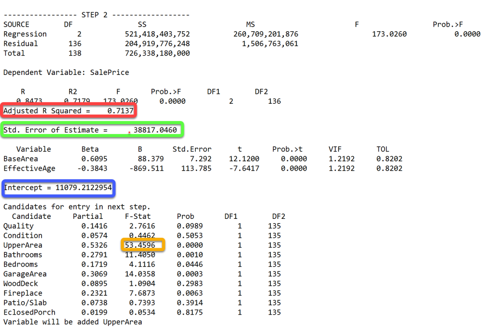
Step 2
Two variables we are looking at to determined sales price:
Base Area
Effective Age (under B has negative number for the adjustment $-869.511) tells us the higher the effective age, the lower the sales price.

Intercept (where we start) $11079
Adjusted R-Squared went up .7137 (that’s good)
Standard Estimate of Error came down 38817 (that’s good)

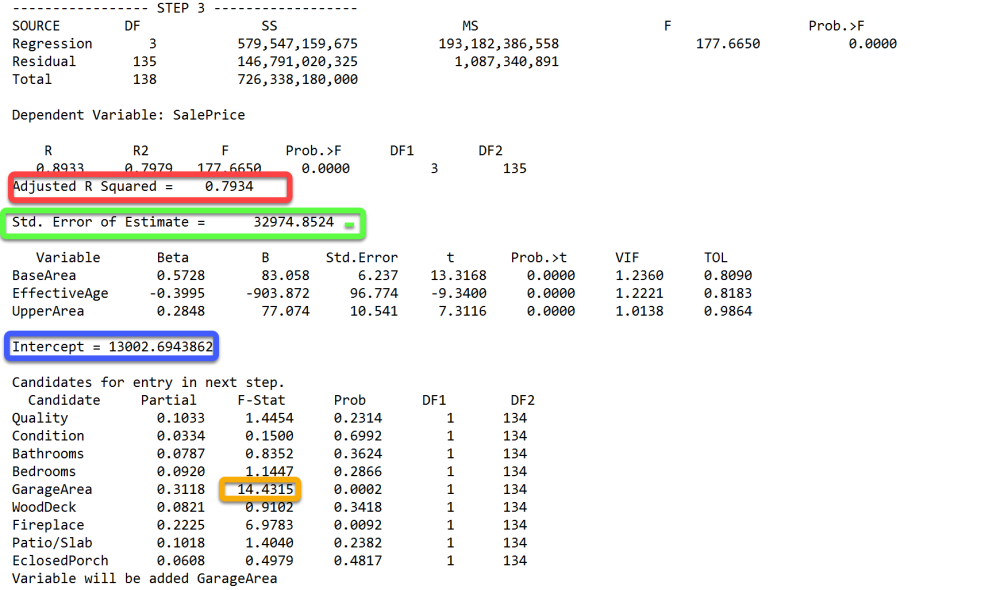
Step 3
Three variables we are looking at to determine sales price:
Base Area
Effective Age
Upper Area

Intercept (where we start) $13002
Adjusted R-Squared went up .7934 (that’s good)
Standard Estimate of Error came down $32974 (that’s good)

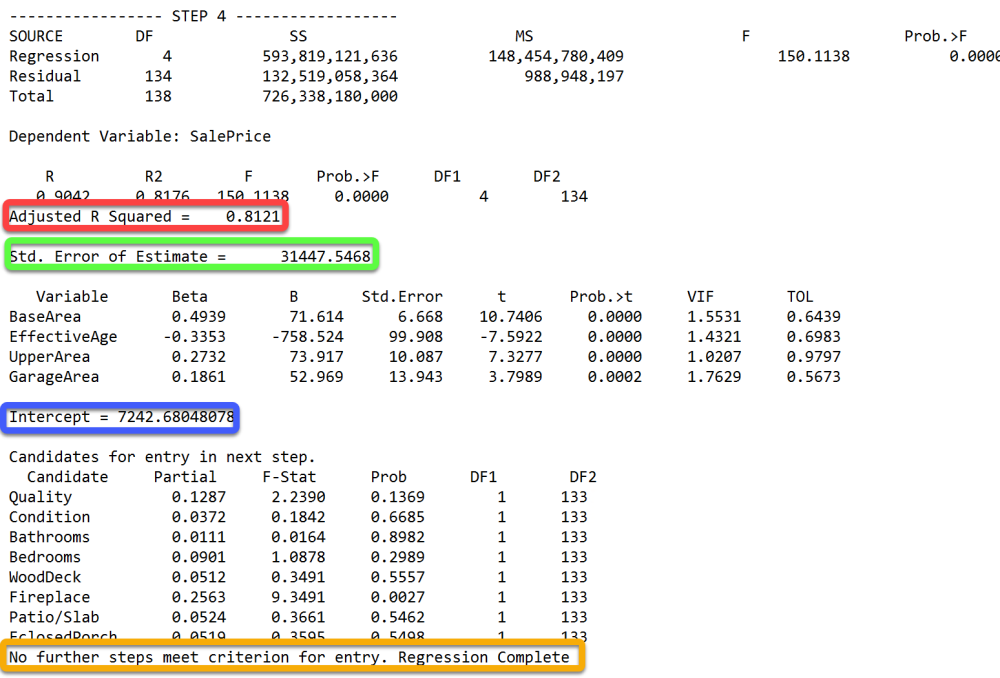
Step Four
Four areas to determine sales price.
Base Area
Effective Age
Upper Area
Garage Area

Intercept (where we start) $7242 (every house starts at this price and is adjusted from there)
Adjusted R-Squared went up .8121 (that’s good)
Standard Estimate of Error came down 38817 (that’s good)

Final Step

Forcing Independent Variables Into/Out of the Model

The user may Edit the model by making it using Variables that were thrown out (or put into) the Analysis. To do this:

• CLICK the Edit Button
• CHECK or UNCHECK the In Model Box of variable to include or not
• CLICK the Down Arrow and CHOOSE Forced-In/Forced-Out (Under Control).
  By forcing variables into an equation, user may try to obtain data in how much to adjust for an attribute in the cost approach. Be careful in doing this.
  

Viewing Multiple Regression Analysis in Excel
User may choose to SAVE and view the MRA in Excel.
Add Fields to include. Example: Account number, total value, neighborhood…

This will show how WELL the model is explaining or predicting sales.

In this example, it will show what the sales price was and what the predicted value is.

To Save Models
Tools — Models — Save Last Model

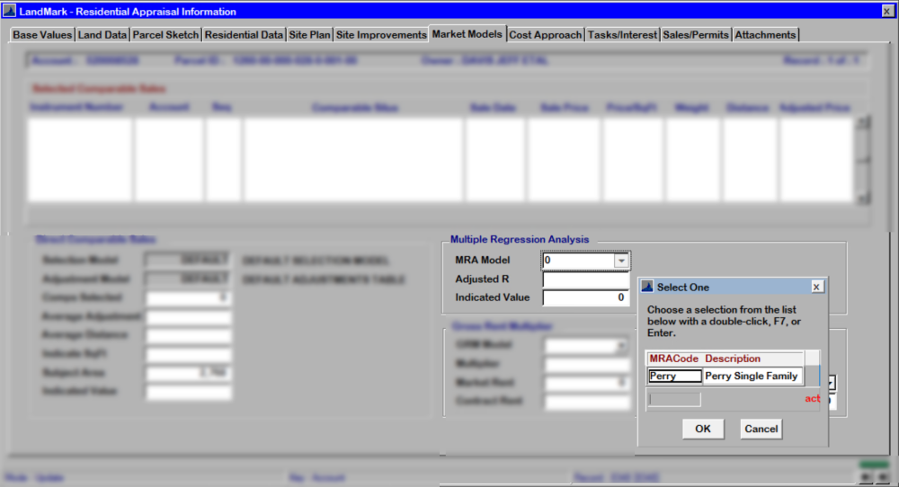
To Apply the Model to a Property.
Appraisal File — Market Model (7th Tab) — Edit Button — Down arrow to Select MRA Code — OK
Indicated Value: is the value that the model is predicting (this value will also show up on the first tab (Base Values)

To view calculations of a model on
View — MRA Model

Discussion on MRA

Question: Should MRA ever be used to determine value?

Answer: If your model fits your sales properties well, Regression will give you THE BEST INDICATOR OF VALUE. However, if you use it, you have to explain it to the tax payer, so it may be a better tool in how much to adjust in the sales approach OR Validate OR show user a problem with the Cost Approach.