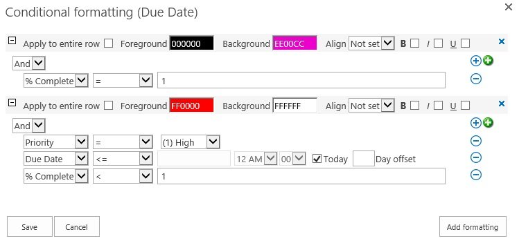
Conditional Formatting

Conditional Formatting can be applied to a cell value or to an entire row of data. You can set the following properties:

• Apply to Entire Row (Without setting this, your formatting is set to the column value only).
• Foreground Color (Select a color or enter the RGB code)
• Background Color (Select a color or enter the RGB code)
• Set the alignment to Not set (default, Left, Center, Right, Justified.
• Select Bold, Italic, Underline checkboxes.
  

To apply condition formatting:

1. Select And or Or and then click the blue plus icon .
2. Select the column which is to be tested. Only those columns you have selected on the Columns tab
3. Set the operator, such as, =, >, <, >= . The operators displayed depend on the column type, for example, for a text column, the operators are Begins with, Contains, =, <>, Is Null and Is Not Null.
4. Set the value.
5. Remove conditions by clicking the Remove condition icon.
6. To define multiple conditions for the same formatting, click the green cross icon .
7. To add a sub condition, click the blue plus icon
8. To define multiple conditional formatting click the Add Formatting button, for example, if you want to format Completed Tasks as Pink and High Priority tasks, that are not completed and whose Due Date has passed, as Red.
   

*Depending on the data type of the column, you may see different properties available such as Today for a Date/Time column type and Me for a User column type.